Linear Decision Boundary by a Perceptron
Perceptron
The Perceptron is the first generation of neural networks. It was modeled to emulate the learning behaviour of our brain.
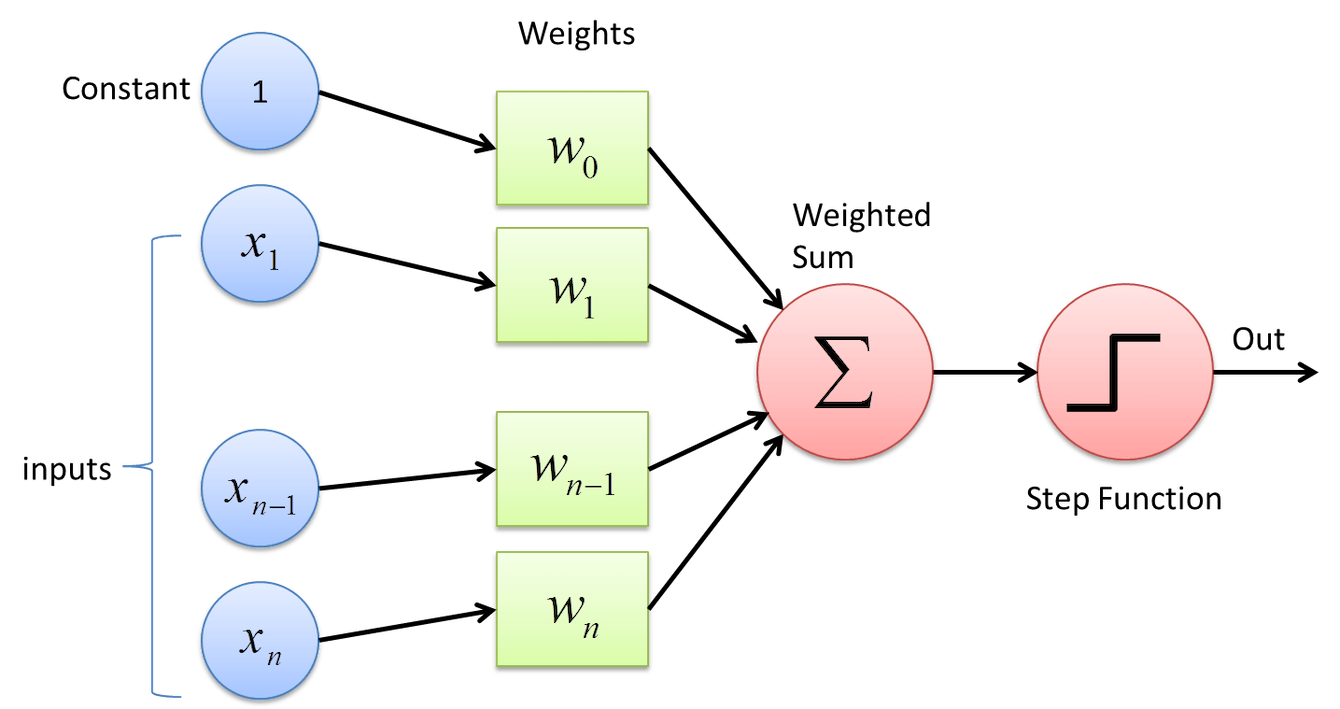
A perceptron can be visualized as follows:

The blue nodes are the inputs to the neuron.
The green nodes are the weights that are learned by the Perceptron algorithm.
The Weighted Sum
Consider the above diagram, we have, $n + 1$ inputs and $n + 1$ corresponding weights.
The weighted sum refers to the process of multiplying the $i$th input to it's corresponding $i$th weight, i.e.
$$ \begin{align} x_{0} * w_{0} + x_{1} * w_{1} + x_{2} * w_{2} + ... + x_{n} * w_{n} \end{align} $$Weighted Sum
$ \begin{align} z = \sum_{i=0}^{i=n} x_{i}w_{i} \end{align} $
Notice that the first input is 1, which boils the equation down to
$ \begin{align} z = \sum_{i=1}^{i=n} x_{i}w_{i} + w_{0} \end{align} $
The $w_{0}$ term is called as bais term as is often written as $b$
$ \begin{align} z = \sum_{i=1}^{i=n} x_{i}w_{i} + b \end{align} $
The Activation function
Finally the result of the above summation is run through a function (typically non-linear), this function is know as the activation function.
Their main purpose is to convert an input signal of a neuron in the Perceptron network to an output signal. This output signal is then used to make a decision about the class that the input pattern belongs to.
In the above diagram, the activation function is defined as follows:
$$ \begin{align} \text{g}(z) = \begin{cases} 1 & \text{if} \ z \ge \theta \\ 0 & \text{otherwise} \\ \end{cases} \end{align} $$The above funtion is know as the Heaviside step function.
The decision boundary
Consider two vector that each belong to a different class(say A and B). The Perceptron can be used to classify them into their respective classes.
We can say that the input vector belongs to the,class A if it fires(the output of the activation function is high) otherwise, it belongs to class B.
%load_ext autoreload
%autoreload 2
from figures import figure1
# Point 1, it will be the red line and belong to class 0
p1 = [10, -8]
# Point 2, it will be the blue line and belong to class 1
p2 = [10, 5]
figure1.draw([p1, p2])
The green line is the weight vector learned $w^{*}$
Decision boundary for AND and OR
from figures import and_boundary
and_boundary.fit()
from figures import or_boundary
or_boundary.fit()