Approximating functions using Sigmoid Perceptrons
In Multi-layer Feed Forward neural networks, you can observe a new found capability of a perceptron network to learn non-linearly separable data sets. You have witnessed that networks with 2 or more layers can learn a non-linear decision boundary.
Here, you will be presented with an example, which aims to show, how a function can be approximated using the Sigmoid.
Before we continue, this is how a sigmoid looks like
from Figures import Sigmoid
Sigmoid.draw()
Approximating functions with Sigmoid
Let us consider, we want to approximate the following function
$$ \begin{align} f(x) = \begin{cases} 1 \ \ \text{if } 2 \le x \le 6 \\ 0 \ \ \text{Otherwise} \end{cases} \end{align} $$from Figures import f
f.draw()

We can use sigmoid with large weights to approximate the above function like so...
Consider the sigmoid used as show below
from Figures import approx1
approx1.draw()

As you can notice a good portion of the function is approximated. But, a single perceptron is not enough. Why?
The above Sigmoid outputs a 1 for all values of x that are approximately greater than 2. We would need another sigmoid perceptron to check the second boundary($x \le 6$).
We make use of a perceptron with negative large weights ...
from Figures import approx2
approx2.draw()

Now, the above perceptron would give us all the points that have the value of x approximately less than 6
from Figures import approx3
approx3.draw()

A good portion of the function has now been approximated. We have used two perceptrons to approximate the function, but we also need a third Perceptron to comibine the results of the two. We need a perceptron that does the AND operation.
We require a total of 3 Perceptrons
The above function approximation can be depicted as the below neural network architecture
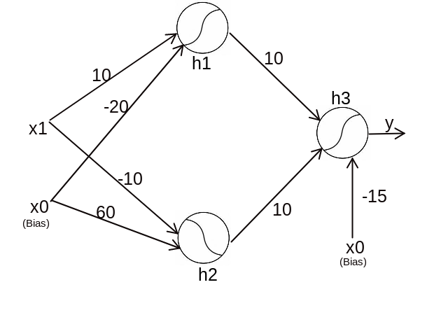 Now let us see in detail how it works.
At $h_1$:
$10\thinspace x_1-20\thinspace x_0 \thinspace > \thinspace 0 \implies 10 \thinspace x_1 -20 \thinspace > \thinspace 0 $ [Since, $x_0$ = 1 because it is bias].
The above equation is satisfied $\forall x \in (2,\infty)$
At $h_2$:
$-10\thinspace x_1+60\thinspace x_0 \thinspace > \thinspace 0 \implies -10 \thinspace x_1 +60 \thinspace > \thinspace 0 $ [Since, $x_0$ = 1 because it is bias].
The above equation is satisfied $\forall x \in (-\infty,6)$
At $h_3$:
$10\thinspace h_1+10\thinspace h_2 -15\thinspace x_0 \thinspace > \thinspace 0 \implies 10\thinspace h_1+10\thinspace h_2 \thinspace > \thinspace 15$ [Since, $x_0$ = 1 because it is bias].
The above equation is satisfied only when both h1 and h2 values evaluate to one. That means this node with the weight and bias values of 10 and -15 respectively acts as an AND gate